
Embeddings - What They Are and How AI Understands Text Meaning

How is it possible for an AI model to know that "samochód" and "auto" mean the same thing, even though they do not share a single letter? This is made possible by embeddings - numerical vector representations of text, in which words and concepts with similar meanings are converted into dense vectors of numbers (most often 300-1024 dimensions) located close to each other in a multidimensional space. As a result, natural language processing does not rely on comparing letters, but rather on semantic similarity measured by metrics such as cosine similarity.
Embeddings are the foundation of text embedding models - from classic Word2Vec, GloVe, and FastText to contextual architectures based on Transformers, such as BERT. This article explains what the process of generating vectors from text looks like, how static vectorization differs from dynamic contextual embeddings, and how this enables a computer to understand meaning, not just the form of words.
Why computers need numbers to understand human language
Computers operate exclusively on numbers - a processor does not "read" the word "cat", but instead performs operations on its numerical representation. AI's understanding of text therefore boils down to converting words, phrases, and documents into embeddings - dense vectors of floating-point numbers of a fixed length that encode content, tone, sentiment, topic, as well as semantic and syntactic relationships.
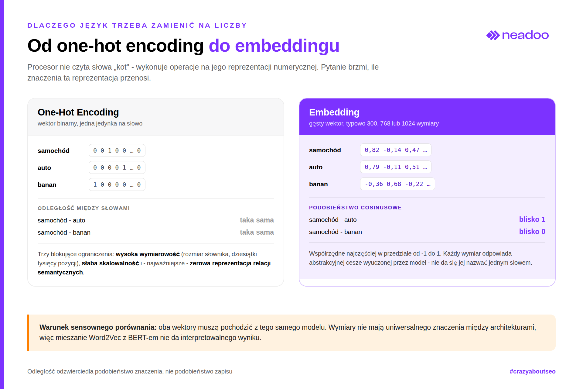
Before modern embeddings were created, the standard was One-Hot Encoding - a method that assigns each word a unique binary vector where only a single position has a value of 1, and all others are 0. This approach suffered from three blocking limitations: high vector dimensionality (size equal to the number of words in the vocabulary, often tens or hundreds of thousands of positions), poor scalability with large vocabularies, and - most importantly - a complete lack of representation of semantic relationships. Under this method, the vectors for "car" and "automobile" were just as distant as the vectors for "car" and "banana".
The next stage of evolution was recurrent neural networks (RNNs), especially their refined version - LSTM (Long Short-Term Memory), designed to retain information from longer text spans. Despite this progress, traditional RNN/LSTM units analyzed context primarily in one direction - most often left-to-right, word by word. This unidirectional flow of information made it difficult to fully understand a sentence, as the meaning of a word depends just as heavily on what follows it as on what precedes it.
These two limitations - the lack of semantics in One-Hot Encoding and the unidirectionality of context in LSTMs - determined the direction for the further development of embedding models, described in subsequent parts of this article. Today, the practical consequences of this evolution extend beyond natural language processing alone - semantic text understanding mechanisms are used, among others, in AI SEO, where search engines evaluate how well content matches user intent at the level of meaning, not just phrase matching.
Step by step: how converting text into numerical vectors works
Text vectorization consists of splitting text into tokens and then processing them with a language model to generate a vector of a specific dimensionality. The process takes place in two stages: first tokenization, then computations in a neural network - this second stage is resource-intensive and significantly slower than the subsequent comparison of finished embeddings, which involves simple mathematical operations.
Tokenization vs. vector text representation
Tokenization is the first and essential step of any vectorization - converting words, word pieces, or characters into numerical identifiers (tokens) that the model accepts as input.
- Text splitting - a tokenization algorithm (e.g., WordPiece, BPE) splits a sentence into units smaller than a whole word, allowing it to handle previously unseen compound words or neologisms.
- Mapping to identifiers - each token receives a unique number from the model's vocabulary; it is this number, not the word itself, that is passed further into the neural network.
- The basis of vector representation - without tokenization, there is no entry point into the model. A neural network operates exclusively on numbers, not on alphabet characters.
Generating vectors using language models
After tokenization, a token reaches the layers of the neural network, where weights (parameters learned from massive text corpora) transform it into a sequence of floating-point numbers.
- Space dimension - the resulting vector has a fixed number of coordinates, typically 300, 768, or 1024. Each dimension corresponds to one abstract semantic or syntactic feature learned by the model.
- Vector coordinates - the values at individual positions most often fall within the range of -1 to 1, making it possible to encode complex, multi-layered semantic features of text into a single point in a multidimensional space.
- Final output - the result is a dense vector representation of the text, in which documents with similar meanings occupy neighboring positions in the multidimensional space, regardless of the words used or their grammatical form.
The evolution of text embedding models: from static vocabularies to contextual BERT
The evolution of text embedding models unfolded across four stages: from static vocabulary representations (Word2Vec, GloVe), through a model that accounts for morphology (FastText), to an architectural breakthrough (Transformer) and the fully contextual BERT model.
| Model | Year | Principle of operation | Key limitation / feature |
|---|---|---|---|
| Word2Vec | 2013 | Google predictive model, trained using CBOW and Skip-gram algorithms | Enables vector operations (king - man + woman ≈ queen), but does not account for context and polysemy |
| GloVe | 2014 | Global word co-occurrence analysis in a corpus and co-occurrence matrix factorization | Static vector per word; requires more memory than Word2Vec |
| FastText | 2016 | Word representation as a sum of character n-gram vectors (subwords) | Handles out-of-vocabulary words and languages with complex morphology |
| Transformer | 2017 | Attention mechanism analyzing the full context of a sentence in parallel | Parallelization of computations, no sequential processing like in RNN/LSTM |
| BERT | 2018 | Transformer-based architecture, trained via Masked Language Modeling and Next Sentence Prediction | Dynamic, contextual embeddings - the same word has a different vector depending on its surroundings |
Word2Vec, GloVe, and FastText share one feature: each word has exactly one, unchangeable vector regardless of the context in which it is used. They differ in their training methods. Word2Vec predicts words from a local context window, GloVe factorizes a co-occurrence matrix built on global statistics of the entire corpus, and FastText, as the only one of the three, breaks down a word into character n-grams - as a result, it creates meaningful vectors even for neologisms and typos, marginalizing the out-of-vocabulary problem that Word2Vec and GloVe do not solve.
The breakthrough came with the Transformer architecture (2017). Its attention mechanism weighs the influence of each token in a sentence on every other token simultaneously, instead of processing text sequentially like an LSTM. The parallelization of computations and full access to bidirectional context enabled the creation of the BERT model (Google, 2018). BERT's training consists of two stages: pre-training with Masked Language Modeling (guessing masked words) and Next Sentence Prediction tasks (evaluating whether two sentences logically follow each other), followed by fine-tuning for a specific task. Thanks to this, the word "castle" (Polish: "zamek") gets a different vector in a sentence about a defensive fortress and in a sentence about a zipper - something that no earlier static model could represent.
Let's check your website's potential
Share your website and email - we'll get back to you with a real analysis, no strings attached.
Cosine similarity and the mathematical measurement of text meaning
Artificial intelligence compares the meaning of texts by calculating the cosine similarity between their vectors - a result close to 1 means nearly identical semantic meaning, regardless of the words used. This metric measures the angle between two vectors, not their length, thus describing the orientation of the vectors relative to each other. The cosine similarity value ranges from -1 to 1: 1 means semantically identical documents, 0 means no semantic relationship, and -1 means opposite meanings. It is complemented by cosine distance, calculated as 1 minus the similarity value - the smaller the distance, the closer the two texts are in terms of content.
A meaningful comparison requires one condition: the vectors must come from the same embedding model. The dimensions of the vector space do not have universal meaning across different architectures, so mixing embeddings from Word2Vec and BERT will not produce an interpretable result. The distance between points in this space reflects semantic similarity, not character-level similarity - thanks to this, synonyms such as "car" and "automobile" achieve a high score despite being spelled completely differently.
Cosine similarity remains one of the fundamental metrics in NLP, but it is no longer the only tool for comparing embeddings. Systems from 2024-2026 use Euclidean distance, dot product, and metrics applied in ANN indices of the IP/IVF type in parallel. The choice of a specific function depends on the model architecture and the vector database implementation: some models (e.g., trained with vector normalization) yield identical rankings for cosine and dot product, while others require a metric consistent with the training process. The documentation of an embedding model usually specifies the recommended metric - ignoring it leads to flawed semantic search results, even when the vectors were generated correctly.
Search optimization: Bi-encoder, Cross-encoder, and Re-ranking architecture
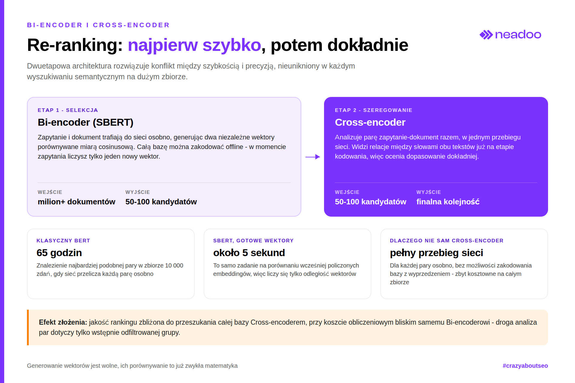
High-performance search systems combine two models: a fast Bi-encoder (SBERT) for the initial selection of documents and a precise Cross-encoder for the final ranking of results (Re-ranking). This two-stage architecture resolves the conflict between speed and precision, typical of any semantic search system operating on large document collections.
Fast selection using a Bi-encoder
- SBERT as the foundation of the Bi-encoder - Sentence-BERT (2019) is a modification of the BERT architecture optimized for generating embeddings of entire sentences rather than individual tokens. The model encodes each text independently, creating a vector ready for comparison without another forward pass through the network.
- Performance leap - comparing pre-computed vectors using cosine similarity shortens the time to find the most similar pair of sentences in a collection of 10,000 sentences from 65 hours (classic BERT comparing each pair separately) to about 5 seconds.
- Principle of operation - the query and the document are fed into the network separately, generating two independent vectors that are then compared using cosine similarity. As a result, the entire document database can be encoded offline and stored as ready-made embeddings, requiring only a single new vector to be calculated at query time.
- Practical application - the Bi-encoder is responsible for the first stage of search: from a million or more documents, it selects a small subset (50-100) of the most promising candidates by searching the vector index.
Precise Re-ranking using a Cross-encoder
- Principle of operation - the Cross-encoder analyzes a pair of texts (query + document) simultaneously by passing them together through a single neural network. The model sees the relationships between the words of both texts already at the encoding stage, which provides a more accurate match score than comparing two separate vectors.
- The cost of precision - simultaneous analysis requires a full forward pass through the network for each text pair, making the Cross-encoder too costly to search the entire document database from scratch.
- Re-ranking architecture - re-ranking combines both models sequentially: the Bi-encoder quickly selects a limited candidate list from the entire collection, and the Cross-encoder precisely ranks this narrowed list, establishing the final order of results.
- End result - the two-stage approach delivers a ranking quality close to searching the entire database with a Cross-encoder, at a computational cost close to that of the Bi-encoder alone - the costly analysis of text pairs applies only to a small, pre-filtered group of documents.
Vector storage and semantic search in RAG systems
Deploying embeddings at scale requires specialized vector databases - they enable lightning-fast searches through millions of records and serve as the foundation of Retrieval-Augmented Generation (RAG) systems. A vector database does not store raw text, but rather its numerical representation along with metadata that allows filtering results and reconstructing the original content once a match is found.
The RAG architecture combines two stages: retrieval of the most relevant knowledge chunks from the database vector database, and generation of the response by a large language model that uses these chunks as additional query context. Thanks to this, RAG solves the fundamental limitation of language models - the lack of access to up-to-date, corporate, or specialized knowledge not covered in the training data. The system does not require fine-tuning the entire model; updating knowledge comes down to replacing the contents of the vector database.
Popular vector databases - Pinecone, Weaviate, Qdrant, Milvus, pgvector, Chroma - differ in their deployment model (managed service vs. self-hosted open-source) and index structure, but they serve the same purpose: minimizing response time while maintaining high result accuracy. For a dataset on the order of 1 million vectors, typical query latencies range from a few to several dozen milliseconds: median (p50) around 9-45 ms, 95th percentile (p95) on the order of 22-89 ms, depending on index configuration and hardware. Such speed is provided by Approximate Nearest Neighbor (ANN) algorithms - HNSW or IVF - which do not compare the query with every vector in the database, but search only a selected graph or cluster structure.

The choice of distance metric in the index must match the metric on which the given embedding model was trained - a mismatch degrades retrieval accuracy even when the database infrastructure operates correctly. Effective implementation of semantic search in RAG - much like other AI visibility efforts - requires simultaneous optimization of embedding model quality, distance metric selection, and ANN index configuration. This is precisely a mistake we see all the time: a team chooses a vector database based on speed benchmarks, and only after deployment discovers that search results are poor because no one checked what metric the embedding model creator recommended.
Semantic quality evaluation using the BERTScore metric
BERTScore evaluates the quality of generated text based on semantic similarity rather than surface word overlap - thanks to this, it provides a more accurate picture of quality than traditional text metrics. The method encodes each token of the candidate and reference sentences using a contextual language model, and then measures the cosine similarity between corresponding fragments in vector space. It therefore does not check whether the text contains words identical to the reference, but whether it conveys the same meaning.
This is where it differs from the classic family of ROUGE metrics, based on matching n-grams and shared word sequences, which penalizes any paraphrasing - even when it preserves the full meaning of the original. BERTScore, operating on token embeddings, recognizes the semantic equivalence of lexically different formulations, e.g., "reduce costs" and "cut expenses," which ROUGE would assign a low score due to the lack of literal word overlap. In research from 2024-2025, ROUGE thus serves as a baseline for evaluating embedding metrics, rather than as a competing metric operating at the same level of abstraction.
Calculating BERTScore does not require additional classifier training on a labeled dataset of human ratings. The method uses ready-made, pre-trained contextual embeddings and matches tokens based on maximum cosine similarity between vector pairs - this is a form of unsupervised learning applied to text evaluation. Thanks to this, BERTScore can be used to evaluate machine translations, summaries, or RAG system responses without building a separate set of reference ratings for each new domain. In our view, it is precisely this ease of implementation - without the stage of building one's own rating dataset - that explains why BERTScore displaced ROUGE from most new evaluation pipelines faster than the difference in metric quality alone would suggest.
Visualization and dimensionality reduction of multidimensional spaces
Dimensionality reduction algorithms - t-SNE, UMAP, and PCA - project multidimensional data onto clear 2D or 3D plots, enabling humans to interpret complex relationships between vectors. Text or graph embeddings usually have from several hundred to several thousand dimensions, which is imperceptible to the human eye. Reduction methods compact this structure while preserving distance and similarity relationships between points to the greatest extent possible.
These methods differ in their mathematical foundation and intended purpose, which translates into different practical applications:
- PCA (Principal Component Analysis) - a linear method that determines directions (principal components) of greatest data variance. It is computationally fast and deterministic. It is well-suited for initial dimensionality reduction prior to further analysis or as a baseline, but poorly reflects non-linear, complex cluster structures in embedding data.
- t-SNE (t-distributed Stochastic Neighbor Embedding) - a non-linear method focusing on preserving local neighborhoods of points: elements similar in the original space remain close to each other after reduction as well. It reveals local semantic clusters well. However, the global distance structure between distant clusters is often distorted, and the result depends on parameters (e.g., perplexity) and random initialization.
- UMAP (Uniform Manifold Approximation and Projection) - a non-linear method based on fuzzy topological set theory. It runs faster than t-SNE and better preserves both local and global data structure, making it a more frequent choice today for visualizing large embedding datasets.
The practical application of these algorithms includes embedding model diagnostics: checking whether documents with similar topics actually form tight clusters in vector space, detecting anomalies or semantic duplicates, and presenting semantic search results in a form understandable to non-technical stakeholders. PCA works well as a quick initial preview or a preprocessing step reducing computational cost before applying t-SNE or UMAP. These latter two methods dominate where faithful reproduction of semantic cluster structure is critical. None of these plots, however, constitutes proof - it is a tool for formulating hypotheses about data structure, not for their definitive confirmation, because dimensionality reduction itself always distorts something.
Graph embeddings as an extension of classic text vectors
Graph embeddings extend vectorization beyond text: they encode the structure of connections within a network, where nodes represent objects (websites, users, documents, products) and edges represent the relationships between them. Node2Vec, the most popular algorithm in this class, generates random walks across the graph and, based on them, learns a vector representation of each node - analogous to language models that learn word representations from their context in text. Nodes that frequently appear close to each other in the generated paths receive similar vectors, even when they are not connected by any direct edge.
Node2Vec builds upon the earlier DeepWalk algorithm, the first to adapt the Word2Vec technique to graph structures by treating random walks as the equivalent of sentences in a text corpus. DeepWalk uses purely random transitions, uniformly selecting the next node from the neighborhood. Node2Vec additionally introduces two parameters (p and q) that control whether the walk prefers exploring the local neighborhood (homophily, structural similarity) or venturing deeper into the graph (discovering structural roles of nodes - such as hubs with a similar function, even if topologically distant). This flexibility allows the representation to be fine-tuned for a specific task: node classification, link prediction, or community detection in a network.
Graph embeddings are used more broadly than just in NLP tasks - they are also applied in the analysis of social networks, scientific citation graphs, link structures between websites, and product-user relationships in recommendation systems. They can be combined with classic text embeddings within a single pipeline: a website can be represented simultaneously by a content vector (semantics) and a position vector within the link graph (structure). Such a combination provides a more complete picture than either representation used alone.
FAQ
What is the difference between static and dynamic embeddings?
Static embeddings (Word2Vec, GloVe, FastText) assign a single, unchangeable vector to a word regardless of context, which makes them unable to handle polysemy. Dynamic embeddings, generated by Transformer-based models (such as BERT), create different vectors for the same word depending on its surrounding context.
How do vector databases speed up semantic search?
They store generated embeddings and optimize similarity calculations (such as cosine similarity) using ANN indexes, enabling semantic search in under 1 second even across millions of entries - generating the vectors themselves is much slower than mathematically comparing them.